Scatterplots Regression
Explanatory & Response Variables
Bivariate Data
- Data that has been collected of two different quantitative variables
Explanatory & Response Variables
Explanatory Variables:
- An explanatory variable is the variable in a set of bivariate data that can be used to predict/explain a response or effect, also referred as independent variables
- On a scatter plot, the explanoatory variable is meausred along the horizontal x-axis
Response Variables:
- The variable in a set of bivariate data whose values are explained by changes in explanatory variable, referred to as dependent variables
Association & Correlation Coeeficients
Association
- Direction of an association
- Positive
- Negative
- Forms of an association
- Linear
- Quadratics, Cubics
- Reciprocals
- Exponentials
- Strength of an association
- Strong
- Moderate
- Weak
- Unusual features of a scatterplot
- Clusters
- Outliers
Correlation Coefficients
Correlation is a numerical measure of the direction and strength of a linear association between two variables
- Correlation coefficient \(r \in [-1, 1]\)
- \(r=1 \implies\) a perfect positive linear
- \(r=-1 \implies\) a perfect negative linear
- \(r=0 \implies\) no linear association
- \(r = \dfrac1{n-1} \sum (\dfrac{x_i - \overline{x}}{s_x})(\dfrac{y_i - \overline{y}}{s_y})\)
- standard deviation of x-values, \(s_x = \sqrt{\dfrac{\sum (x_i - \overline{x})^2}{n-1}}\)
- standard deviation of y-values, \(s_y = \sqrt{\dfrac{\sum (y_i - \overline{y})^2}{n-1}}\)
- Correlation does not imply causation
- If two variables appear to correlate, it does not mean that one variable causes changes in the other variable
Interpolation & Extrapolation using Linear Models
Interpolation & Extrapolation
Interpolation means using a regression line to predict a \(y\)-value from a given \(x\)-value,
where the \(x\)-value lies within the interval of \(x\)-values seen in the data.
- This is seen as a reliable prediction
Extrapolation means using a regression line to predict a \(y\)-value from a given \(x\)-value,
where the \(x\)-value lies outside the interval of \(x\)-values seen in the data.
- This is far less reliable, as you do not know how the variables relate outside the range of data given
- The linear relationship might break down or change direction
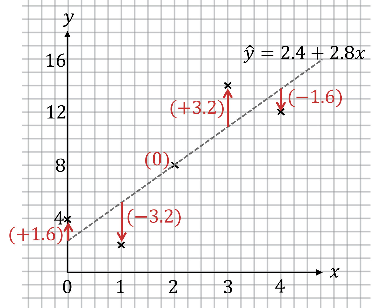
Residuals
Residual = actual \(y\)-value - predicted \(y\)-value
Least-Squares Regression Line
The least-squares regression line is a type of regression line that: > - Minimize the sum of squares of the residuals > - Passes through the mean point \((\overline{x}, \overline{y})\)
- Predict \(y\)-values from given \(x\)-values
-
Cannot swap \(x\) and \(y\)
-
Sum of the squares of the residuals = \(\sum (residual)^2\)
- Equation of the least-squares regression line \(\hat{y} = a + bx\)
- \(\hat{y}\) is the \(y\)-value predicted
- \(x\) is the explanatory variable
- \(a\) is the \(y\)-intercept
- \(b\) is the slope
- note the order of the terms
- Slope \(b = r \dfrac{s_x}{s_y}\)
- \(r\) is the correlation coefficient
- \(\overline{y} = a + b \overline{x}\)
- Can be used to find \(a\), but need to find \(b\) first
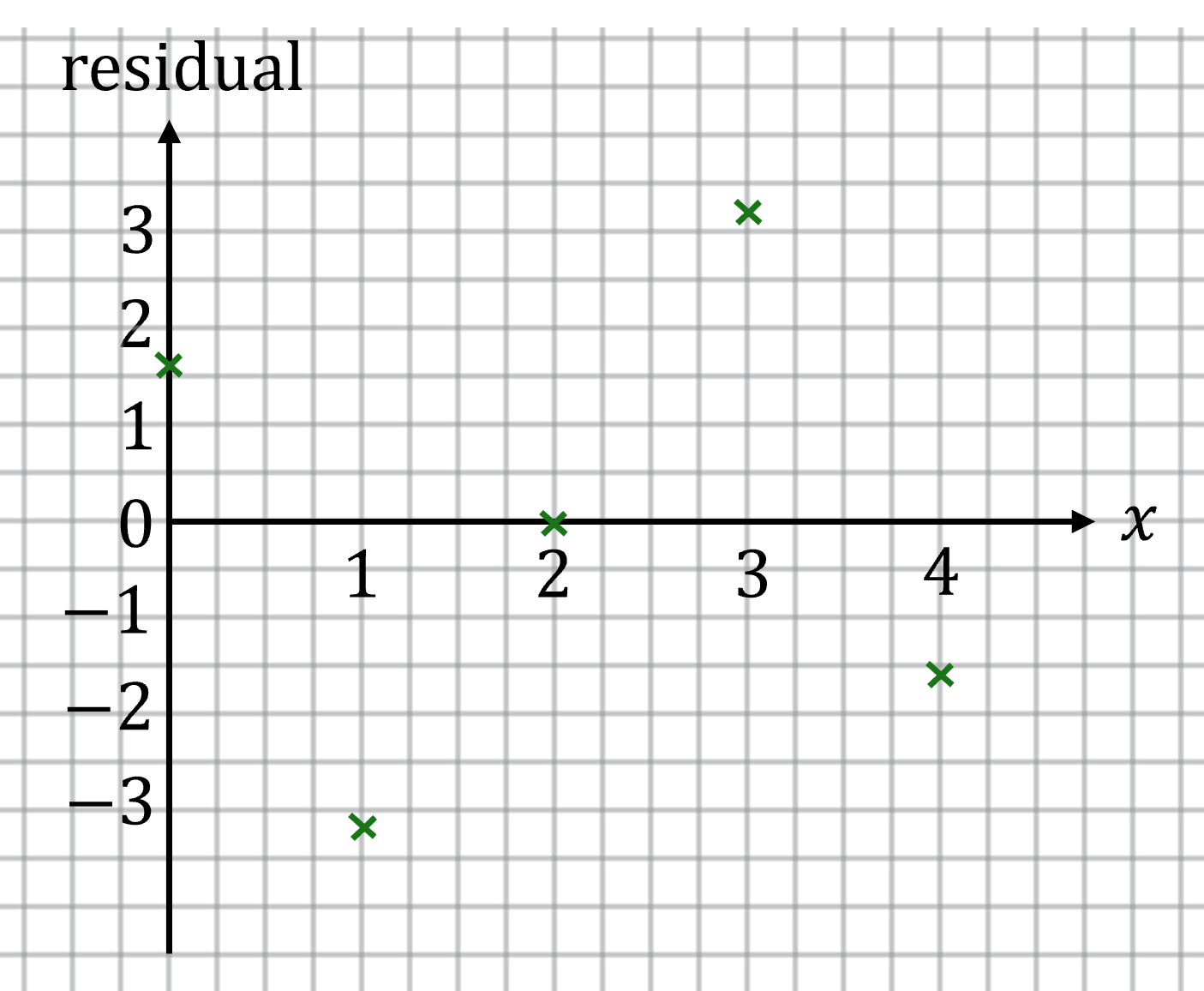
Residual Plots
A residual plot is a graph that shows all the residuals from a scatterplot > - y-axis shows the value of the residual
For a least-squares regression line:
- If the residuals vary randomly from positive to negative, a linear model is a good fit
- If the residuals follow a curve or a pattern, a linear model is not a good fit
\(\rightarrow\)
Coefficient of Determination
The coefficient of determination is the proportion of the total variation in the response variable that is explained by the linear relationship with the explanatory variable.
The coefficient of determination for a least-squares regression line is \(r^2 \in [0, 1]\). Values of \(r^2\) indicate that the regression is a good model for the data.
The coefficient of determination indicates that \([percentage]\) of the total variance in the \([y-variable]\) is explained by the linear relationship with the \(x-variable\).
To get the correlation coefficient from the coefficient of determination, take the square root, then check the least-squares regression line, - If the slope is positive, take the positive square root - If the slope is negative, take the negative square root
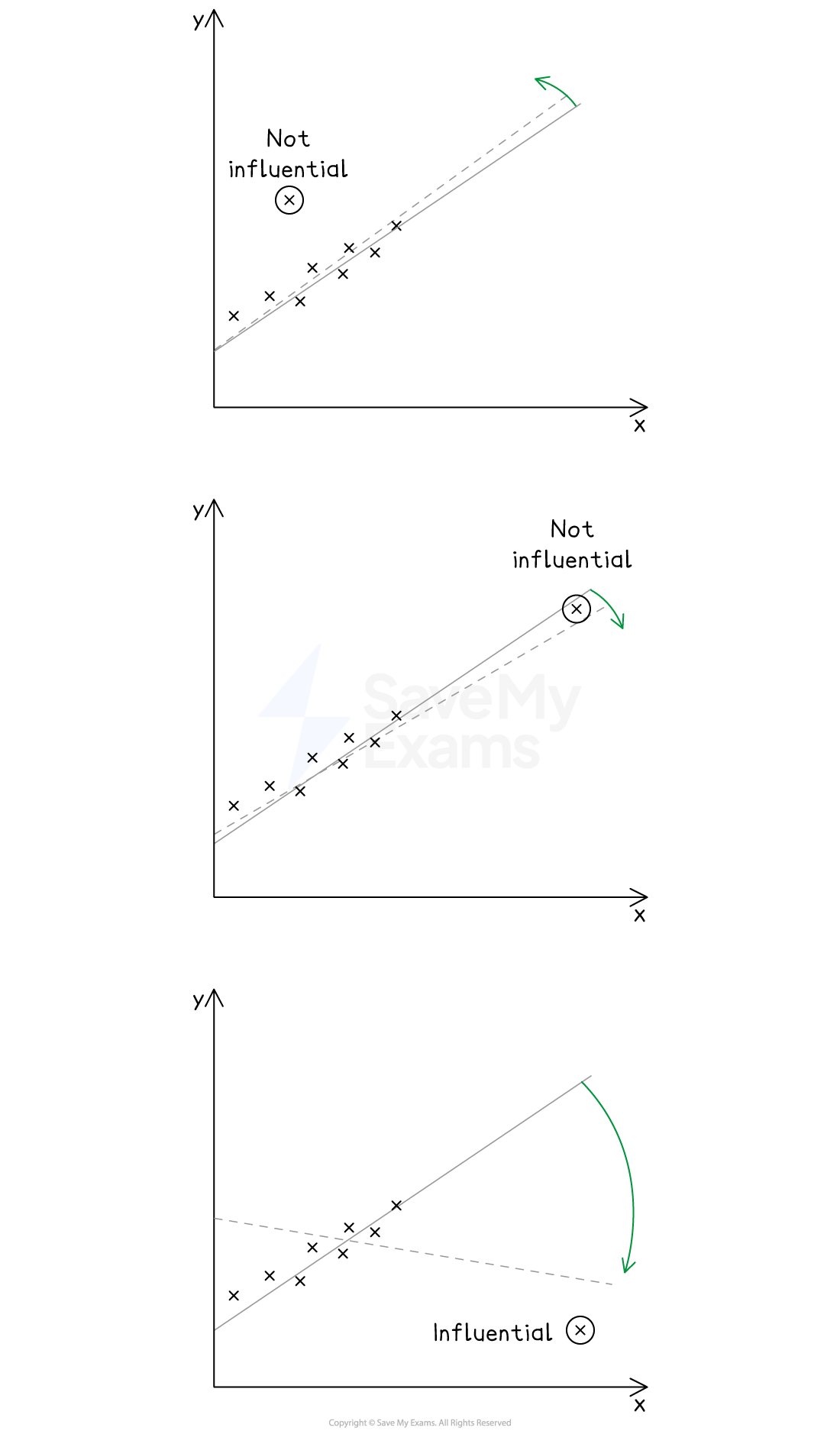
Outliers & High-Leverage & Influential Points
An outlier in a regression model is a point that has an extreme \(y\)-value relative to the least-squares regression line
A high-leverage point is a data point that has an extreme \(x\)-value relative to other data points
A high-leverage point is not an outlier unless its \(y\)-value is extreme to the least-squares regression line
An influential point in a regression model is a model that , if removed, changes the linear relationship significantly
Removing an influential point could cause a significant change in
- the correlation coefficient \(r\)
- the slope of a regression line
- the \(y\)-intercept of a regression line
An outlier that is also a high-leverage point is likely to be an influential point
- An outlier that is also a high-leverage point is likely to be an influential point
- Outliers or high-leverage points alone may or may not be influential points
Linearization of Bivariate Data
Transforming a variable means performing a mathematical operation on either the \(x\)-coordinates of the data points, or the \(y\)-coordinates
There are two different methods to check if the transformed data is more linear than the untransformed data:
- Create residual plots before and after the transformation to evaluate the randomness
- Calculate the coefficient of determination \(r^2\) before and after the transformation to evaluate how close it is to \(1\)