Demand and supply

Supply Curve¶

Determinants of Supply¶

The supply curve illustrates how the quantity supplied responds to changes in various factors. Below is a breakdown of the determinants:

Elasticity Concepts¶

Price Elasticity of Demand (PED)¶

Formula:

Types of Price Elasticity of Demand¶

• Perfectly Elastic Demand $PED = \infty$: The demand curve is a horizontal line.

• Relatively Elastic Demand
  $PED > 1$: Percentage change in quantity demanded exceeds percentage change in price ($\Delta QD\% > \Delta P\%$).

• Unit Elastic Demand
  $PED = 1$: Percentage change in quantity demanded equals percentage change in price ($\Delta QD\% = \Delta P\%$).

• Relatively Inelastic Demand
  $0 < PED < 1$: Percentage change in quantity demanded is less than percentage change in price ($\Delta QD\% < \Delta P\%$).

• Perfectly Inelastic Demand
  $PED = 0$: The demand curve is a vertical line.

Total Revenue and Elasticity¶

• $Price \propto TR \implies \text{Inelastic}$
• $Price \propto \frac{1}{TR} \implies \text{Elastic}$
• $Price = C \implies \text{Unit Elastic}$

2.2 Price Elasticity of Supply (PES)¶

Formula:

Simple Formula¶

• $\Delta \text{Quantity Supplied\%} = \frac{Q_2 - Q_1}{Q_1}$
• $\Delta \text{Price\%} = \frac{P_2 - P_1}{P_1}$

Mid-Point Formula¶

• $\Delta \text{Quantity Supplied\%} = \frac{Q_2 - Q_1}{\frac{Q_2 + Q_1}{2}}$
• $\Delta \text{Price\%} = \frac{P_2 - P_1}{\frac{P_2 + P_1}{2}}$

Types of Price Elasticity of Supply¶

• Perfectly Elastic Supply
  $PES = \infty$: The supply curve is a horizontal line.

• Relatively Elastic Supply
  $PES > 1$: Percentage change in quantity supplied exceeds percentage change in price ($\Delta QS\% > \Delta P\%$).

• Unit Elastic Supply
  $PES = 1$: Percentage change in quantity supplied equals percentage change in price ($\Delta QS\% = \Delta P\%$).

• Relatively Inelastic Supply
  $0 < PES < 1$: Percentage change in quantity supplied is less than percentage change in price ($\Delta QS\% < \Delta P\%$).

• Perfectly Inelastic Supply
  $PES = 0$: The supply curve is a vertical line.

2.3 Income Elasticity of Demand (YED)¶

Formula**: $$ YED = \frac{\Delta \text{Quantity\%}}{\Delta \text{Income\%}} $$

• $YED > 0 \implies \text{Normal Good}$
• $YED < 0 \implies \text{Inferior Good}$

2.4 Cross-Price Elasticity of Demand (XED)¶

Formula:

• $XED > 0 \implies \text{Substitutes}$
• $XED < 0 \implies \text{Complements}$

Market Equilibrium¶

Equilibrium Price¶

The equilibrium price is the point where the Demand Curve and Supply Curve intersect.

Changes in Supply and Demand¶

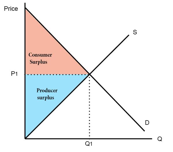
Consumer and Producer Surplus¶

Consumer Surplus¶

• Willingness to Pay (WTP): The maximum price a consumer is willing to pay for a good or service.
• Marginal Buyer: The consumer who leaves the market first if the price rises further.

Producer Surplus¶

• Marginal Seller: The producer who leaves the market first if the price decreases further.

Total Surplus¶

Government Intervention in Markets¶

Price Ceiling¶

• Effective only when actual price > price ceiling.
• Causes a shortage:
  $$ \text{Shortage} = QD - QS $$
• Protects consumers.

Price Floor¶

• Effective only when actual price < price floor.
• Causes a surplus:
  $$ \text{Surplus} = QS - QD $$
• Protects producers.

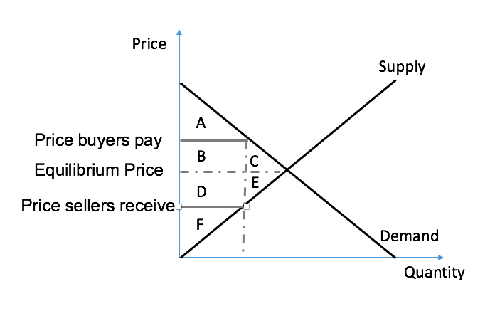
Taxes¶

• Tax burden depends on elasticity:
  $$ \text{Inelastic} \implies \text{Higher tax burden} $$
• Size of tax:
  $$ \text{Size of Tax} = \text{Price of Demand} - \text{Price of Supply} $$
• Tax revenue:
  $$ \text{Tax Revenue} = T \cdot Q $$

Impact of Taxes on Surplus¶

Comments